Basic plot types
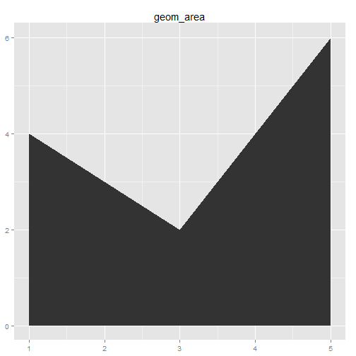
- geom_area() draws an area plot, which is a line plot filled to the y-axis.
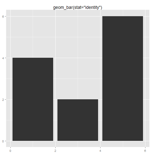
- geom_bar(stat = “identity”)() makes a barchart.
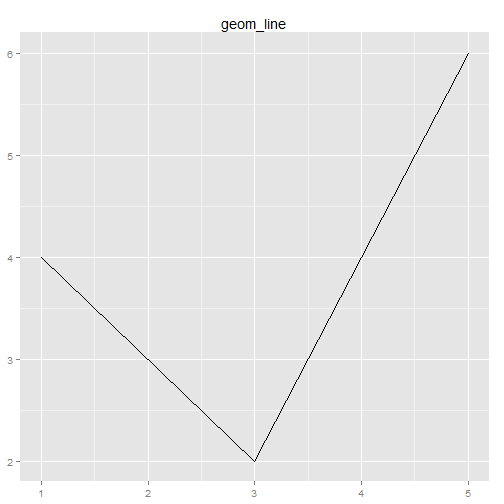
- geom_line() makes a line plot.
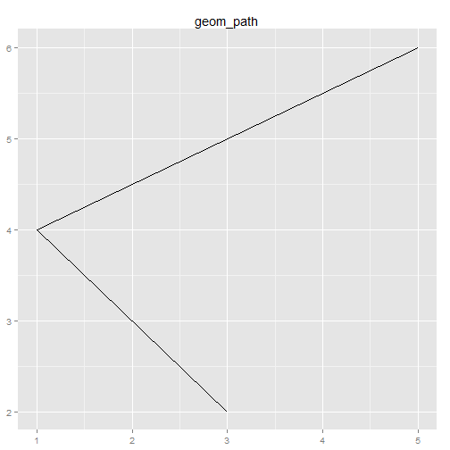
- geom_path() is similar to a geom_line, but lines are connected in the order they appear in the data, not from left to right.
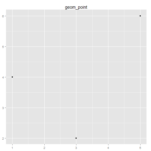
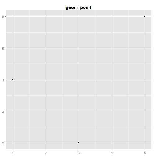
- geom_point() produces a scatterplot.
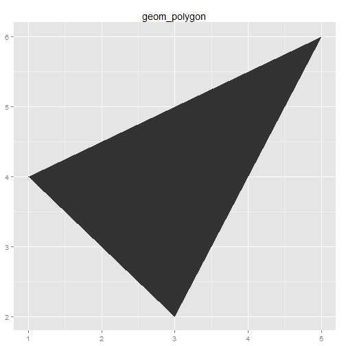
- geom_polygon() draws polygons, which are filled paths.
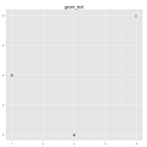
- geom_text() adds labels at the specified points.
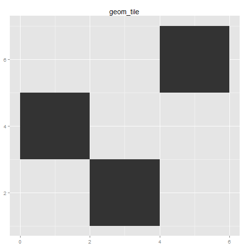
- geom_tile() makes a image plot or level plot.
library(ggplot2)
library(effects)
library(plyr)
diamonds = na.omit(diamonds)

df <- data.frame(x = c(3, 1, 5), y = c(2, 4, 6), label = c("a", "b", "c"))
p <- ggplot(df, aes(x, y, label = label)) + xlab(NULL) + ylab(NULL)
p + geom_point() + labs(title = "geom_point")
# Equivalent to p + geom_point() + ggtitle('geom_point')

# Reduce line spacing and use bold text
p + geom_point() + ggtitle("geom_point") + theme(plot.title = element_text(lineheight = 0.8,
face = "bold"))
p + geom_bar(stat = "identity") + labs(title = "geom_bar(stat=\"identity\")")
p + geom_line() + labs(title = "geom_line")
p + geom_area() + labs(title = "geom_area")
p + geom_path() + labs(title = "geom_path")
p + geom_text() + labs(title = "geom_text")
p + geom_tile() + labs(title = "geom_tile")
p + geom_polygon() + labs(title = "geom_polygon")
Displaying distributions
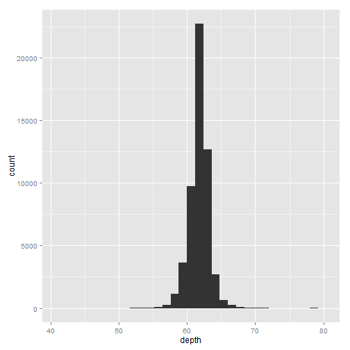
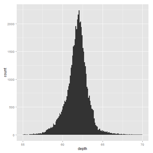
# Never rely on the default parameters to get a revealing view of the
# distribution.  Zooming in on the x axis, and selecting a smaller bin
# width, reveals far more detail.  We can see that the distribution is
# slightly skew-right.  Don't forget to include information about important
# parameters (like bin width) in the caption.
qplot(depth, data = diamonds, geom = "histogram")
qplot(depth, data = diamonds, geom = "histogram", xlim = c(55, 70), binwidth = 0.1)
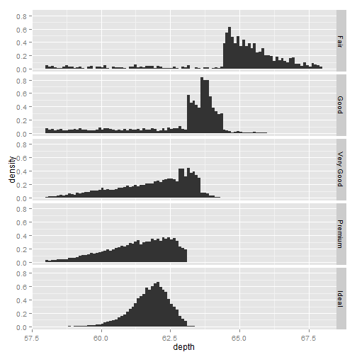
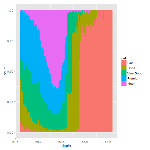
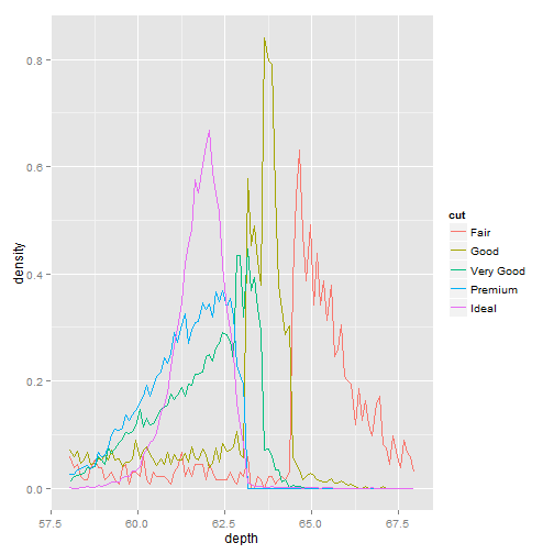
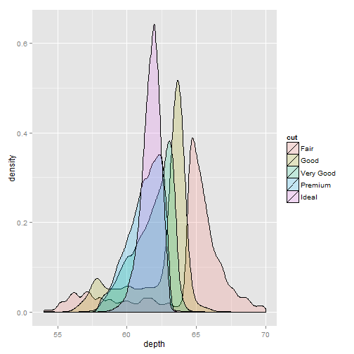
# Three views of the distribution of depth and cut.  faceted histogram, a
# conditional density plot, and frequency polygons.  All show an interesting
# pattern: as quality increases, the distribution shifts to the left and
# becomes more symmetric.
depth_dist <- ggplot(diamonds, aes(depth)) + xlim(58, 68)
depth_dist + geom_histogram(aes(y = ..density..), binwidth = 0.1) + facet_grid(cut ~
.)
depth_dist + geom_histogram(aes(fill = cut), binwidth = 0.1, position = "fill")
depth_dist + geom_freqpoly(aes(y = ..density.., colour = cut), binwidth = 0.1)
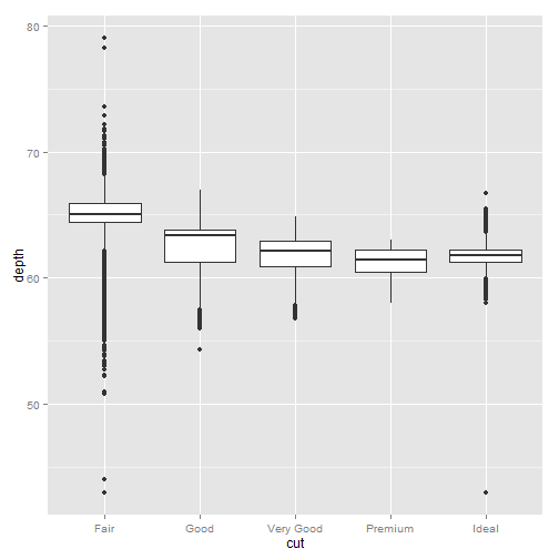
# The boxplot geom can be use to see the distribution of a continuous
# variable conditional on a discrete varable like cut , or continuous
# variable like carat.  For continuous variables, the group aesthetic must
# be set to get multiple boxplots.
qplot(cut, depth, data = diamonds, geom = "boxplot")
qplot(carat, depth, data = diamonds, geom = "boxplot", group = round_any(carat,
0.1, floor), xlim = c(0, 3))

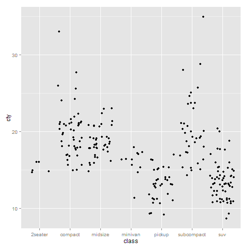
# The jitter geom can be used to give a crude visualisation of 2d
# distributions with a discrete component.  Generally this works better for
# smaller datasets.  Car class vs. continuous variable city mpg and discrete
# variable drive train.
qplot(class, cty, data = mpg, geom = "jitter")
qplot(class, drv, data = mpg, geom = "jitter")

# The density plot is a smoothed version of the histogram. It has desirable
# theoretical properties, but is more difficult to relate back to the data.
# A density plot of depth, coloured by cut
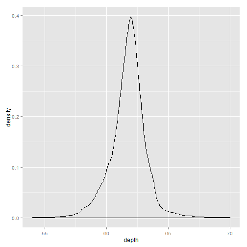
qplot(depth, data = diamonds, geom = "density", xlim = c(54, 70))
qplot(depth, data = diamonds, geom = "density", xlim = c(54, 70), fill = cut,
alpha = I(0.2))
Dealing with overplotting
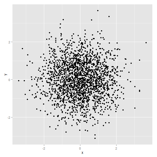
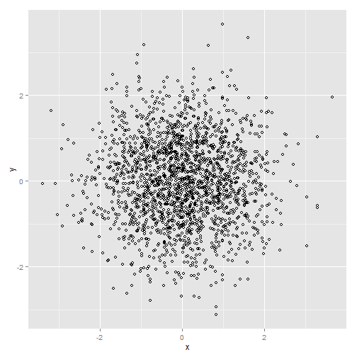
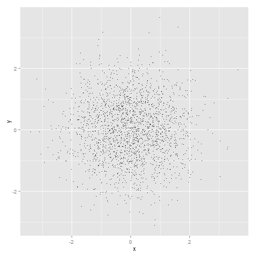
df <- data.frame(x = rnorm(2000), y = rnorm(2000))
norm <- ggplot(df, aes(x, y))
# the default shape
norm + geom_point()
# hollow points
norm + geom_point(shape = 1)
# pixel points
norm + geom_point(shape = ".")
# Using alpha blending to alleviate overplotting in sample data from a
# bivariate normal.  Alpha values from left to right: 1/3, 1/5, 1/10.
norm + geom_point(colour = "black", alpha = 1/3)
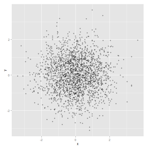
norm + geom_point(colour = "black", alpha = 1/5)
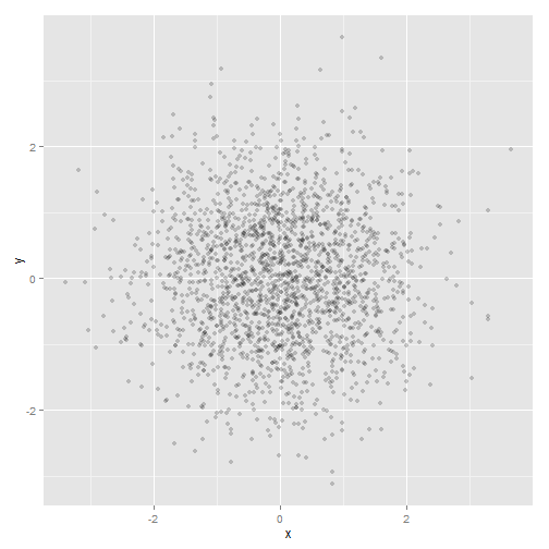
norm + geom_point(colour = "black", alpha = 1/10)

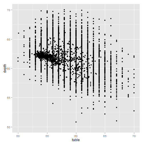
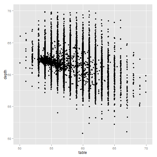
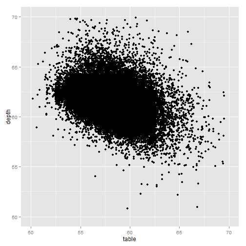
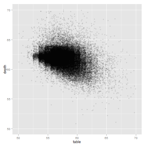
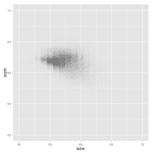
# A plot of table vs. depth from the diamonds data, showing the use of
# jitter and alpha blending to alleviate overplotting in discrete data.
td <- ggplot(diamonds, aes(table, depth)) + xlim(50, 70) + ylim(50, 70)
# geom point
td + geom_point()
# geom jitter with default jitter
td + geom_jitter()
# geom jitter with horizontal jitter of 0.5 (half the gap between bands)
jit <- position_jitter(width = 0.5)
td + geom_jitter(position = jit)
td + geom_jitter(position = jit, colour = "black", alpha = 1/10)
td + geom_jitter(position = jit, colour = "black", alpha = 1/50)
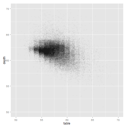
td + geom_jitter(position = jit, colour = "black", alpha = 1/200)
Drawing maps
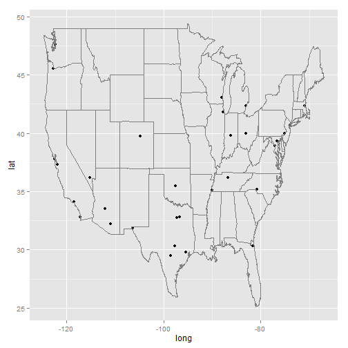
# Example using the borders function.
library(maps)
data(us.cities)
big_cities <- subset(us.cities, pop > 5e+05)
# All cities with population (as of January 2006) of greater than half a
# million
qplot(long, lat, data = big_cities) + borders("state", size = 0.5)
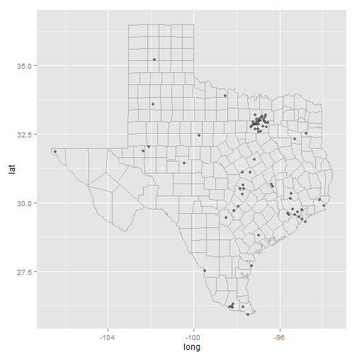
# cities in Texas.
tx_cities <- subset(us.cities, country.etc == "TX")
ggplot(tx_cities, aes(long, lat)) + borders("county", "texas", colour = "grey70") +
geom_point(colour = "black", alpha = 0.5)
Further reading