ggplot2 part 3

library(ggplot2)
data(Oxboys, package = "nlme")
diamonds = na.omit(diamonds)
msleep = na.omit(msleep)
mtcars = na.omit(mtcars)
Oxboys = na.omit(Oxboys)
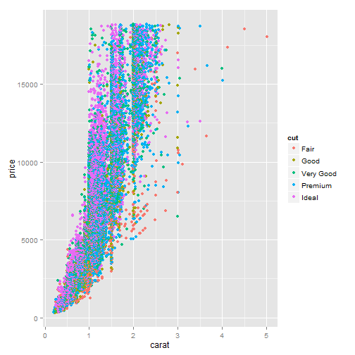
p <- ggplot(diamonds, aes(carat, price, colour = cut))
# This plot object cannot be displayed until we add a layer
p <- p + layer(geom = "point")
p

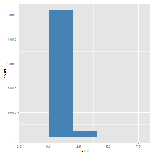
# Here is what a more complicated call looks like.  It produces a histogram
# coloured “steelblue” with a bin width of 2 histogram is a combination of
# bars and binning
p <- ggplot(diamonds, aes(x = carat))
p <- p + layer(geom = "bar", geom_params = list(fill = "steelblue"), stat = "bin",
stat_params = list(binwidth = 2))
p

# same as the following command
ggplot(diamonds, aes(x = carat)) + geom_histogram(binwidth = 2, fill = "steelblue")

# The following example shows the equivalence between these two ways of
# making plots

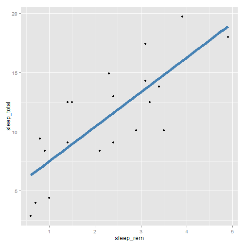
ggplot(msleep, aes(sleep_rem/sleep_total, awake)) + geom_point()
# which is equivalent to
qplot(sleep_rem/sleep_total, awake, data = msleep)

# You can add layers to qplot too:
qplot(sleep_rem/sleep_total, awake, data = msleep) + geom_smooth()
# This is equivalent to
qplot(sleep_rem/sleep_total, awake, data = msleep, geom = c("point", "smooth"))
# or
ggplot(msleep, aes(sleep_rem/sleep_total, awake)) + geom_point() + geom_smooth()

# plot objects can be stored as variables. The summary function can be
# helpful for inspecting the structure of a plot without plotting it
p <- ggplot(msleep, aes(sleep_rem/sleep_total, awake))
summary(p)

p <- p + geom_point()
summary(p)

# a set of plots can be initialised using different data then enhanced with
# the same layer

bestfit <- geom_smooth(method = "lm", se = F, colour = "steelblue", alpha = 0.5,
size = 2)

qplot(sleep_rem, sleep_total, data = msleep) + bestfit

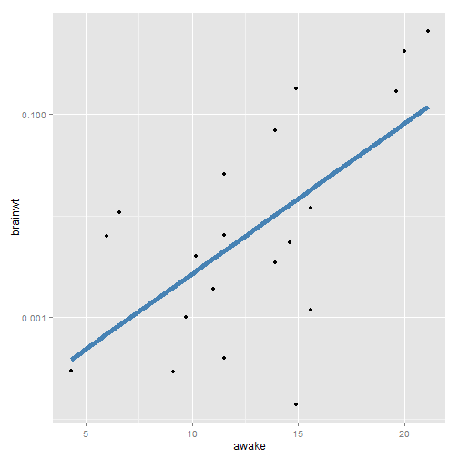
qplot(awake, brainwt, data = msleep, log = "y") + bestfit

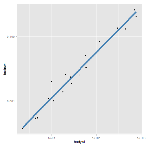
qplot(bodywt, brainwt, data = msleep, log = "xy") + bestfit

# You can replace the old dataset with %+%
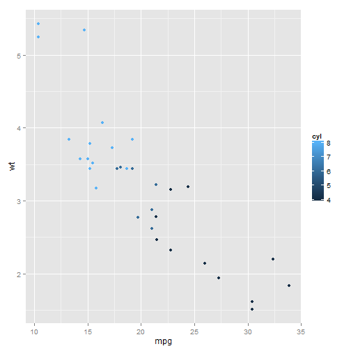
p <- ggplot(mtcars, aes(mpg, wt, colour = cyl)) + geom_point()
p

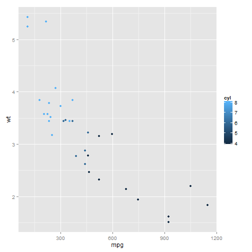
mtcars <- transform(mtcars, mpg = mpg^2)
p %+% mtcars

# The **aes** function takes a list of aesthetic-variable pairs aes(x =
# weight, y = height, colour = age)
p <- ggplot(mtcars, aes(x = mpg, y = wt))
p + geom_point()

# Overriding aesthetics.
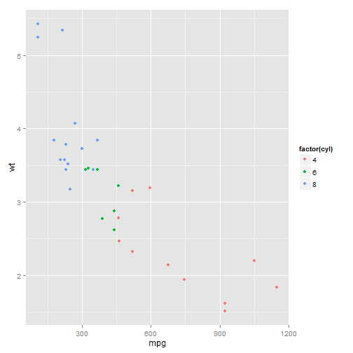
p + geom_point(aes(colour = factor(cyl)))

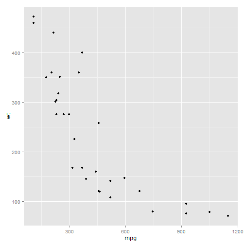
# overriding y-position (now y is 'disp',although the y lab is still 'wt')
p + geom_point(aes(y = disp))

# The difference between setting colour to 'darkblue' and mapping colour to
# 'darkblue'.
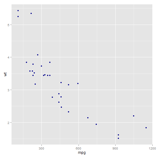
p <- ggplot(mtcars, aes(mpg, wt))
p + geom_point(colour = "darkblue")  # setting

# This sets the point colour to be dark blue instead of black. This is quite
# different than
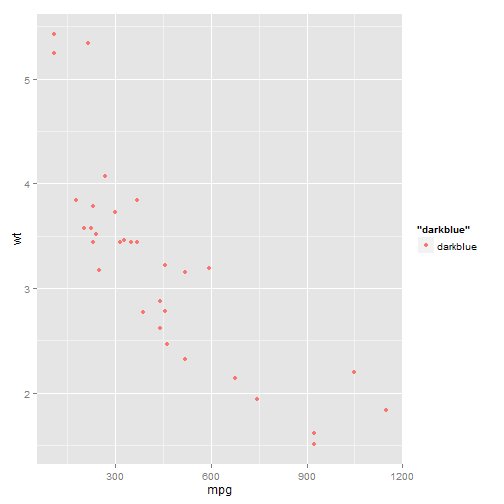
p + geom_point(aes(colour = "darkblue"))  # mapping

# qplot
qplot(mpg, wt, data = mtcars, colour = I("darkblue"))  # setting
qplot(mpg, wt, data = mtcars, colour = "darkblue")  # mapping

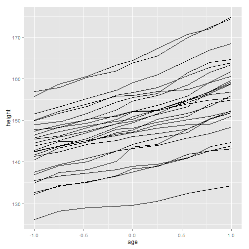
# Correctly specifying produces one line per subject.
p <- ggplot(Oxboys, aes(age, height, group = Subject)) + geom_line()
p

qplot(age, height, data = Oxboys, group = Subject, geom = "line")

# A single line connects all observations.  This pattern is characteristic
# of an **incorrect** grouping aesthetic, and is what we see if the group
# aesthetic is omitted, which in this case is equivalent to group = 1
ggplot(Oxboys, aes(age, height, group = 1)) + geom_line()

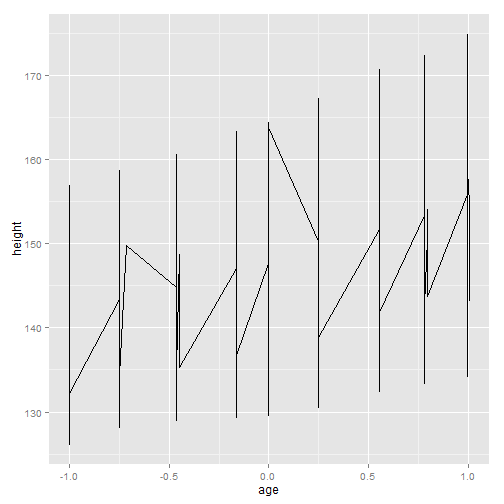
qplot(age, height, data = Oxboys, geom = "line")

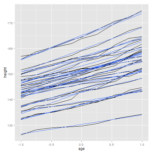
# Adding smooths to the Oxboys data. Using the same grouping as the lines
# results in a line of best fit for each boy.
p + geom_smooth(aes(group = Subject), method = "lm", se = F)

# or
qplot(age, height, data = Oxboys, group = Subject, geom = "line") + geom_smooth(method = "lm",
se = F)

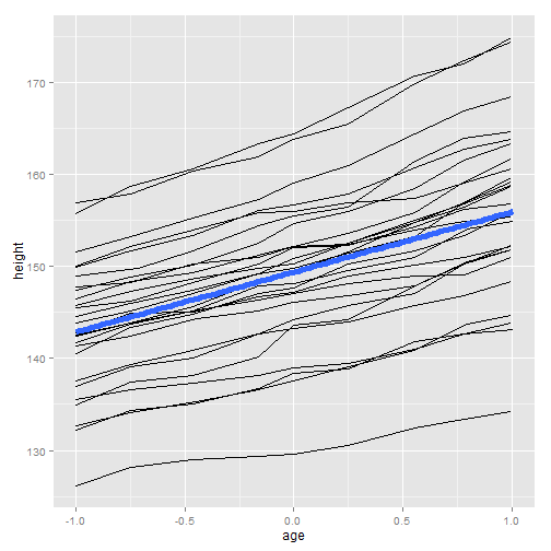
# Using aes(group = 1) in the smooth layer fits a single line of best fit
# across all boys.
p + geom_smooth(aes(group = 1), method = "lm", size = 2, se = F)

qplot(age, height, data = Oxboys, group = Subject, geom = "line") + geom_smooth(aes(group = 1),
method = "lm", size = 2, se = F)