Download data
library(FinCal)

# history data from start (1993) to today
SPY <- get.ohlc.yahoo("SPY")
head(SPY)
date  open  high   low close  volume adjusted
5308 1993-01-29 43.97 43.97 43.75 43.94 1003200    29.78
5307 1993-02-01 43.97 44.25 43.97 44.25  480500    29.99
5306 1993-02-02 44.22 44.38 44.13 44.34  201300    30.05
5305 1993-02-03 44.41 44.84 44.38 44.81  529400    30.37
5304 1993-02-04 44.97 45.09 44.47 45.00  531500    30.50
5303 1993-02-05 44.97 45.06 44.72 44.97  492100    30.48
# adjusted closing prices
SPY.Close <- SPY$adjusted
SPY.vector <- as.vector(SPY.Close)

# Calculate log returns
sp500 <- diff(log(SPY.vector), lag = 1)

# Remove the NA in the first position
sp500 <- sp500[-1]
head(sp500)
[1] 0.001999 0.010593 0.004271 -0.000656 0.000000 -0.006914
Compute the first four moments of the data
library(GLDEX)

# output is the set of estimated lambda parameters λ1 through λ4 for both
# the RS version and the FMKL version of the GLD.
spLambdaDist = fun.data.fit.mm(sp500)
spLambdaDist
RPRS     RMFMKL
[1,]  4.711e-04  4.038e-04
[2,] -4.381e+01  2.081e+02
[3,] -1.700e-01 -1.723e-01
[4,] -1.662e-01 -1.635e-01
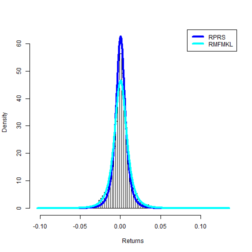
# histogram plot of the data along with the density curves for the RS and
# FMKL fits
fun.plot.fit(fit.obj = spLambdaDist, data = sp500, nclass = 100, param.vec = c("rs",
"fmkl"), xlab = "Returns")
Simulate returns using parameters generated by last step
# RS parameters
lambda.params.rs <- spLambdaDist[, 1]
lambda1.rs <- lambda.params.rs[1]
lambda2.rs <- lambda.params.rs[2]
lambda3.rs <- lambda.params.rs[3]
lambda4.rs <- lambda.params.rs[4]

# RS simulation
set.seed(999)
rs.sample <- rgl(n = 1e+07, lambda1 = lambda1.rs, lambda2 = lambda2.rs, lambda3 = lambda3.rs,
lambda4 = lambda4.rs, param = "rs")

# FKML parameters
lambda.params.fmkl <- spLambdaDist[, 2]
lambda1.fmkl <- lambda.params.fmkl[1]
lambda2.fmkl <- lambda.params.fmkl[2]
lambda3.fmkl <- lambda.params.fmkl[3]
lambda4.fmkl <- lambda.params.fmkl[4]

# FKML simulation
set.seed(999)
fmkl.sample <- rgl(n = 1e+07, lambda1 = lambda1.fmkl, lambda2 = lambda2.fmkl,
lambda = lambda3.fmkl, lambda4 = lambda4.fmkl, param = "fmkl")
Comparing results for the RS, FKML simulation vs S&P 500 market data
# Set normalise='Y' so that kurtosis is calculated with reference to
# kurtosis = 0 under Normal distribution

# Moments of simulated returns using RS method:
fun.moments.r(rs.sample, normalise = "Y")
mean   variance   skewness   kurtosis
3.418e-04  9.457e-05 -1.027e-01  9.947e+00
# Moments of simulated returns using FMKL method:
fun.moments.r(fmkl.sample, normalise = "Y")
mean   variance   skewness   kurtosis
0.0003415  0.0001481 -0.1029554  9.9199126
# Moments calculated from market data:
fun.moments.r(sp500, normalise = "Y")
mean   variance   skewness   kurtosis
0.0003428  0.0001477 -0.1056554  9.9116401
FKML gets better results especially for skewness and variance. Compare to two parameters normal distribution, four parameters generalized lambda distribution is able to preserve skewness and kurtosis of the observed data.
For more details, read the original post here