Data
library(RCurl)
myCsv <- getURL("https://dl.dropboxusercontent.com/u/8272421/stat/stat_one.txt",
ssl.verifypeer = FALSE)
mydata <- read.csv(textConnection(myCsv), sep = "\t")
mydata$subject <- factor(mydata$subject)
Create two subsets, control and concussed
concussed <- subset(mydata, condition == "concussed")
control <- subset(mydata, condition == "control")
Summary statistics
library(psych)
describe(mydata)
var  n  mean    sd median trimmed   mad   min
subject*                      1 40 20.50 11.69  20.50   20.50 14.83  1.00
condition*                    2 40  1.50  0.51   1.50    1.50  0.74  1.00
verbal_memory_baseline        3 40 89.75  6.44  91.00   90.44  6.67 75.00
visual_memory_baseline        4 40 74.88  8.60  75.00   74.97  9.64 59.00
visual.motor_speed_baseline   5 40 34.03  3.90  33.50   34.02  3.62 26.29
reaction_time_baseline        6 40  0.67  0.15   0.65    0.66  0.13  0.42
impulse_control_baseline      7 40  8.28  2.05   8.50    8.38  2.22  2.00
total_symptom_baseline        8 40  0.05  0.22   0.00    0.00  0.00  0.00
verbal_memory_retest          9 40 82.00 11.02  85.00   82.97  9.64 59.00
visual_memory_retest         10 40 71.90  8.42  72.00   72.19 10.38 54.00
visual.motor_speed_retest    11 40 35.83  8.66  35.15   34.98  6.89 20.15
reaction_time_retest         12 40  0.67  0.22   0.65    0.65  0.13  0.19
impulse_control_retest       13 40  6.75  2.98   7.00    6.81  2.97  1.00
total_symptom_retest         14 40 13.88 15.32   7.00   12.38 10.38  0.00
max range  skew kurtosis   se
subject*                    40.00 39.00  0.00    -1.29 1.85
condition*                   2.00  1.00  0.00    -2.05 0.08
verbal_memory_baseline      98.00 23.00 -0.70    -0.51 1.02
visual_memory_baseline      91.00 32.00 -0.11    -0.96 1.36
visual.motor_speed_baseline 41.87 15.58  0.08    -0.75 0.62
reaction_time_baseline       1.20  0.78  1.14     2.21 0.02
impulse_control_baseline    12.00 10.00 -0.57     0.36 0.32
total_symptom_baseline       1.00  1.00  3.98    14.16 0.03
verbal_memory_retest        97.00 38.00 -0.65    -0.81 1.74
visual_memory_retest        86.00 32.00 -0.28    -0.87 1.33
visual.motor_speed_retest   60.77 40.62  0.86     0.65 1.37
reaction_time_retest         1.30  1.11  0.93     1.29 0.03
impulse_control_retest      12.00 11.00 -0.16    -1.06 0.47
total_symptom_retest        43.00 43.00  0.44    -1.47 2.42
describeBy(mydata, mydata$condition)
group: concussed
var  n  mean    sd median trimmed   mad   min
subject*                      1 20 30.50  5.92  30.50   30.50  7.41 21.00
condition*                    2 20  1.00  0.00   1.00    1.00  0.00  1.00
verbal_memory_baseline        3 20 89.65  7.17  92.50   90.56  5.93 75.00
visual_memory_baseline        4 20 74.75  8.03  74.00   74.25  8.15 63.00
visual.motor_speed_baseline   5 20 33.20  3.62  33.09   33.27  3.32 26.29
reaction_time_baseline        6 20  0.66  0.17   0.63    0.64  0.13  0.42
impulse_control_baseline      7 20  8.55  1.64   9.00    8.62  1.48  5.00
total_symptom_baseline        8 20  0.05  0.22   0.00    0.00  0.00  0.00
verbal_memory_retest          9 20 74.05  9.86  74.00   73.88 11.86 59.00
visual_memory_retest         10 20 69.20  8.38  69.50   69.62 10.38 54.00
visual.motor_speed_retest    11 20 38.27 10.01  35.15   37.32  7.73 25.70
reaction_time_retest         12 20  0.78  0.23   0.70    0.74  0.11  0.51
impulse_control_retest       13 20  5.00  2.53   5.00    4.88  2.97  1.00
total_symptom_retest         14 20 27.65  9.07  27.00   27.75 11.12 13.00
max range  skew kurtosis   se
subject*                    40.00 19.00  0.00    -1.38 1.32
condition*                   1.00  0.00   NaN      NaN 0.00
verbal_memory_baseline      97.00 22.00 -0.79    -0.70 1.60
visual_memory_baseline      91.00 28.00  0.45    -0.72 1.80
visual.motor_speed_baseline 39.18 12.89 -0.13    -0.78 0.81
reaction_time_baseline       1.20  0.78  1.38     2.41 0.04
impulse_control_baseline    11.00  6.00 -0.39    -0.81 0.37
total_symptom_baseline       1.00  1.00  3.82    13.29 0.05
verbal_memory_retest        91.00 32.00  0.07    -1.24 2.21
visual_memory_retest        80.00 26.00 -0.27    -1.26 1.87
visual.motor_speed_retest   60.77 35.07  0.77    -0.57 2.24
reaction_time_retest         1.30  0.79  1.09    -0.10 0.05
impulse_control_retest      11.00 10.00  0.39    -0.28 0.57
total_symptom_retest        43.00 30.00 -0.11    -1.25 2.03
--------------------------------------------------------
group: control
var  n  mean   sd median trimmed  mad   min
subject*                      1 20 10.50 5.92  10.50   10.50 7.41  1.00
condition*                    2 20  2.00 0.00   2.00    2.00 0.00  2.00
verbal_memory_baseline        3 20 89.85 5.82  90.00   90.31 7.41 78.00
visual_memory_baseline        4 20 75.00 9.34  77.00   75.50 9.64 59.00
visual.motor_speed_baseline   5 20 34.86 4.09  34.39   34.85 4.92 27.36
reaction_time_baseline        6 20  0.67 0.13   0.66    0.67 0.13  0.42
impulse_control_baseline      7 20  8.00 2.41   7.50    8.12 2.22  2.00
total_symptom_baseline        8 20  0.05 0.22   0.00    0.00 0.00  0.00
verbal_memory_retest          9 20 89.95 4.36  90.50   90.06 5.19 81.00
visual_memory_retest         10 20 74.60 7.76  74.50   75.00 8.15 60.00
visual.motor_speed_retest    11 20 33.40 6.44  34.54   33.52 6.30 20.15
reaction_time_retest         12 20  0.57 0.16   0.56    0.57 0.13  0.19
impulse_control_retest       13 20  8.50 2.31   9.00    8.69 1.48  3.00
total_symptom_retest         14 20  0.10 0.31   0.00    0.00 0.00  0.00
max range  skew kurtosis   se
subject*                    20.00 19.00  0.00    -1.38 1.32
condition*                   2.00  0.00   NaN      NaN 0.00
verbal_memory_baseline      98.00 20.00 -0.41    -0.87 1.30
visual_memory_baseline      88.00 29.00 -0.46    -1.27 2.09
visual.motor_speed_baseline 41.87 14.51  0.09    -1.19 0.91
reaction_time_baseline       1.00  0.58  0.47    -0.02 0.03
impulse_control_baseline    12.00 10.00 -0.41    -0.17 0.54
total_symptom_baseline       1.00  1.00  3.82    13.29 0.05
verbal_memory_retest        97.00 16.00 -0.25    -1.02 0.97
visual_memory_retest        86.00 26.00 -0.23    -1.11 1.73
visual.motor_speed_retest   44.28 24.13 -0.25    -0.77 1.44
reaction_time_retest         0.90  0.71 -0.16     0.06 0.04
impulse_control_retest      12.00  9.00 -0.73    -0.32 0.52
total_symptom_retest         1.00  1.00  2.47     4.32 0.07
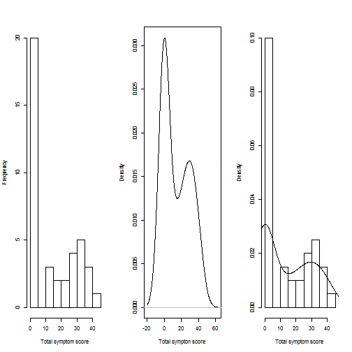
Density plots
par(mfrow = c(1, 3))
hist(mydata$total_symptom_retest, xlab = "Total symptom score", main = "")
plot(density(mydata$total_symptom_retest), xlab = "Total sympton score", main = "")

# prob=TRUE for probabilities not counts
hist(mydata$total_symptom_retest, xlab = "Total symptom score", main = "", prob = TRUE)
lines(density(mydata$total_symptom_retest))
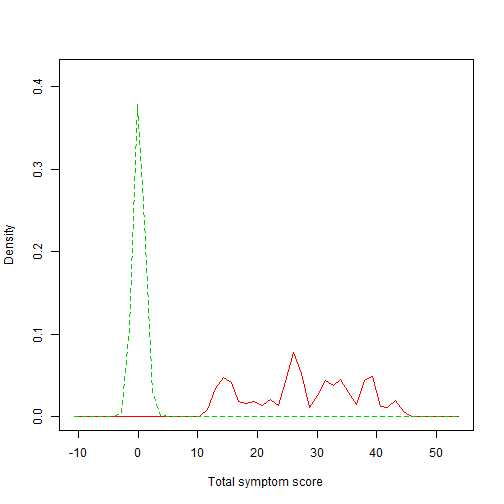
Compare density plots
library(sm)
par(mfrow = c(1, 1))
# This function allows a set of univariate density estimates to be compared,
# both graphically and formally in a permutation test of equality.
sm.density.compare(mydata$total_symptom_retest, mydata$condition, xlab = "Total symptom score")
Correlation analysis of baseline measures
cor(mydata[3:8]) # Columns 3 to 8 contain the 6 baseline measures
verbal_memory_baseline visual_memory_baseline
verbal_memory_baseline                     1.00000                0.37512
visual_memory_baseline                     0.37512                1.00000
visual.motor_speed_baseline               -0.04057               -0.23339
reaction_time_baseline                     0.14673                0.13615
impulse_control_baseline                   0.13147                0.23756
total_symptom_baseline                     0.13521                0.01689
visual.motor_speed_baseline
verbal_memory_baseline                        -0.040567
visual_memory_baseline                        -0.233391
visual.motor_speed_baseline                    1.000000
reaction_time_baseline                        -0.131955
impulse_control_baseline                       0.005221
total_symptom_baseline                        -0.051903
reaction_time_baseline
verbal_memory_baseline                      0.1467
visual_memory_baseline                      0.1361
visual.motor_speed_baseline                -0.1320
reaction_time_baseline                      1.0000
impulse_control_baseline                    0.1213
total_symptom_baseline                     -0.0339
impulse_control_baseline
verbal_memory_baseline                      0.131471
visual_memory_baseline                      0.237559
visual.motor_speed_baseline                 0.005221
reaction_time_baseline                      0.121334
impulse_control_baseline                    1.000000
total_symptom_baseline                      0.082149
total_symptom_baseline
verbal_memory_baseline                     0.13521
visual_memory_baseline                     0.01689
visual.motor_speed_baseline               -0.05190
reaction_time_baseline                    -0.03390
impulse_control_baseline                   0.08215
total_symptom_baseline                     1.00000
round(cor(mydata[3:8]), 2) # Round to 2 decimal places
verbal_memory_baseline visual_memory_baseline
verbal_memory_baseline                        1.00                   0.38
visual_memory_baseline                        0.38                   1.00
visual.motor_speed_baseline                  -0.04                  -0.23
reaction_time_baseline                        0.15                   0.14
impulse_control_baseline                      0.13                   0.24
total_symptom_baseline                        0.14                   0.02
visual.motor_speed_baseline
verbal_memory_baseline                            -0.04
visual_memory_baseline                            -0.23
visual.motor_speed_baseline                        1.00
reaction_time_baseline                            -0.13
impulse_control_baseline                           0.01
total_symptom_baseline                            -0.05
reaction_time_baseline
verbal_memory_baseline                        0.15
visual_memory_baseline                        0.14
visual.motor_speed_baseline                  -0.13
reaction_time_baseline                        1.00
impulse_control_baseline                      0.12
total_symptom_baseline                       -0.03
impulse_control_baseline
verbal_memory_baseline                          0.13
visual_memory_baseline                          0.24
visual.motor_speed_baseline                     0.01
reaction_time_baseline                          0.12
impulse_control_baseline                        1.00
total_symptom_baseline                          0.08
total_symptom_baseline
verbal_memory_baseline                        0.14
visual_memory_baseline                        0.02
visual.motor_speed_baseline                  -0.05
reaction_time_baseline                       -0.03
impulse_control_baseline                      0.08
total_symptom_baseline                        1.00
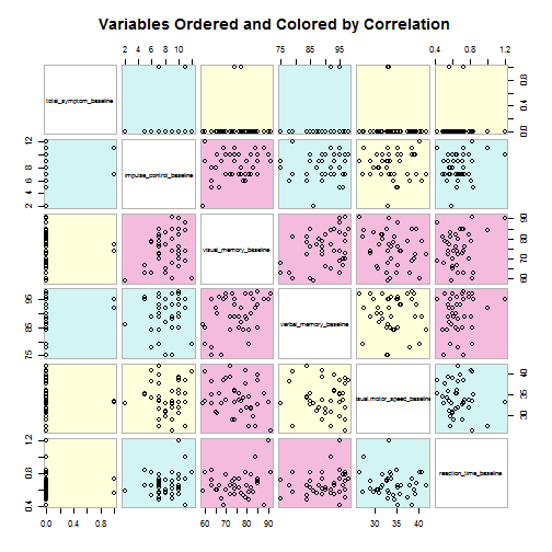
Color scatterplot matrix, colored and ordered by magnitude of r
library(gclus)
base <- mydata[3:8]
base.r <- abs(cor(base))
base.color <- dmat.color(base.r)
base.order <- order.single(base.r)
# This function draws a scatterplot matrix of data.  Variables may be
# reordered and panels colored in the display
cpairs(base, base.order, panel.colors = base.color, gap = 0.5, main = "Variables Ordered and Colored by Correlation")
Regression analyses, unstandardized
model1 <- lm(mydata$visual_memory_retest ~ mydata$visual_memory_baseline)
summary(model1)
Call:
lm(formula = mydata$visual_memory_retest ~ mydata$visual_memory_baseline)

Residuals:
Min     1Q Median     3Q    Max
-8.137 -2.553 -0.358  2.803 12.152


Coefficients:
Estimate Std. Error t value Pr(>|t|)
(Intercept)                    10.3386     6.5090    1.59     0.12
mydata$visual_memory_baseline   0.8222     0.0864    9.52  1.3e-11 ***
---
Signif. codes:  0 '***' 0.001 '**' 0.01 '*' 0.05 '.' 0.1 ' ' 1

Residual standard error: 4.64 on 38 degrees of freedom
Multiple R-squared:  0.705,	Adjusted R-squared:  0.697
F-statistic: 90.6 on 1 and 38 DF,  p-value: 1.32e-11
# Print 95% confidence interval for the regression coefficient
confint(model1)
2.5 %  97.5 %
(Intercept)                   -2.8381 23.5154
mydata$visual_memory_baseline  0.6473  0.9971
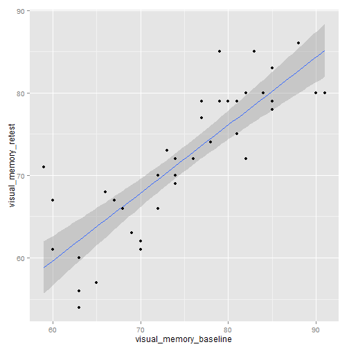
# Scatterplot with confidence interval around the regression line
library(ggplot2)
ggplot(mydata, aes(x = visual_memory_baseline, y = visual_memory_retest)) +
geom_smooth(method = "lm") + geom_point()
par(mfrow = c(1, 1))
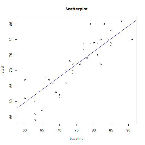
plot(mydata$visual_memory_retest ~ mydata$visual_memory_baseline, main = "Scatterplot",
ylab = "retest", xlab = "baseline")
abline(model1, col = "blue")
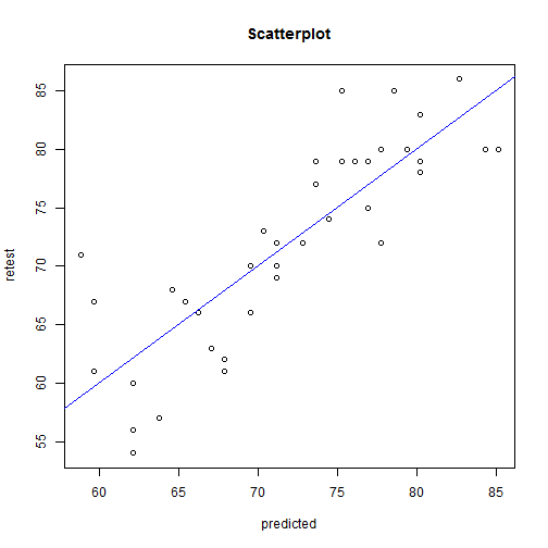
# To visualize model1, save the predicted scores as a new variable and then
# plot with endurance
mydata$predicted <- fitted(model1)
par(mfrow = c(1, 1))
plot(mydata$visual_memory_retest ~ mydata$predicted, main = "Scatterplot", ylab = "retest",
xlab = "predicted")
abline(lm(mydata$visual_memory_retest ~ mydata$predicted), col = "blue")
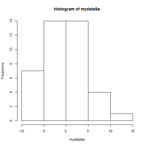
# The function fitted returns predicted scores whereas the function resid
# returns residuals
mydata$e <- resid(model1)
hist(mydata$e)
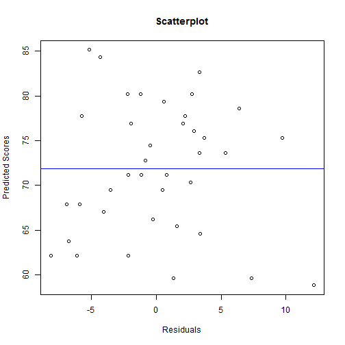
plot(mydata$predicted ~ mydata$e, main = "Scatterplot", ylab = "Predicted Scores",
xlab = "Residuals")
abline(lm(mydata$predicted ~ mydata$e), col = "blue")
# Conduct a model comparison NHST to compare the fit of model1 to the fit of
# model2
model2 <- lm(mydata$visual_memory_retest ~ mydata$visual_memory_baseline + mydata$verbal_memory_baseline)
anova(model1, model2)
Analysis of Variance Table

Model 1: mydata$visual_memory_retest ~ mydata$visual_memory_baseline
Model 2: mydata$visual_memory_retest ~ mydata$visual_memory_baseline +
mydata$verbal_memory_baseline
Res.Df RSS Df Sum of Sq   F Pr(>F)
1     38 818
2     37 790  1      27.8 1.3   0.26
Regression analyses, standardized
# In simple regression, the standardized regression coefficient will be the
# same as the correlation coefficient

round(cor(mydata[3:5]), 2)  # Round to 2 decimal places
verbal_memory_baseline visual_memory_baseline
verbal_memory_baseline                        1.00                   0.38
visual_memory_baseline                        0.38                   1.00
visual.motor_speed_baseline                  -0.04                  -0.23
visual.motor_speed_baseline
verbal_memory_baseline                            -0.04
visual_memory_baseline                            -0.23
visual.motor_speed_baseline                        1.00
model1.z <- lm(scale(mydata$verbal_memory_baseline) ~ scale(mydata$visual_memory_baseline))
summary(model1.z)
Call:
lm(formula = scale(mydata$verbal_memory_baseline) ~ scale(mydata$visual_memory_baseline))

Residuals:
Min      1Q  Median      3Q     Max
-1.9891 -0.5813  0.0866  0.7885  1.3377


Coefficients:
Estimate Std. Error t value Pr(>|t|)
(Intercept)                          -2.63e-17   1.48e-01    0.00    1.000
scale(mydata$visual_memory_baseline)  3.75e-01   1.50e-01    2.49    0.017

(Intercept)
scale(mydata$visual_memory_baseline) *
---
Signif. codes:  0 '***' 0.001 '**' 0.01 '*' 0.05 '.' 0.1 ' ' 1

Residual standard error: 0.939 on 38 degrees of freedom
Multiple R-squared:  0.141,	Adjusted R-squared:  0.118
F-statistic: 6.22 on 1 and 38 DF,  p-value: 0.0171
model2.z <- lm(scale(mydata$verbal_memory_baseline) ~ scale(mydata$visual.motor_speed_baseline))
summary(model2.z)
Call:
lm(formula = scale(mydata$verbal_memory_baseline) ~ scale(mydata$visual.motor_speed_baseline))

Residuals:
Min     1Q Median     3Q    Max
-2.302 -0.730  0.146  0.826  1.327


Coefficients:
Estimate Std. Error t value
(Intercept)                               -1.85e-17   1.60e-01    0.00
scale(mydata$visual.motor_speed_baseline) -4.06e-02   1.62e-01   -0.25
Pr(>|t|)
(Intercept)                                    1.0
scale(mydata$visual.motor_speed_baseline)      0.8

Residual standard error: 1.01 on 38 degrees of freedom
Multiple R-squared:  0.00165,	Adjusted R-squared:  -0.0246
F-statistic: 0.0626 on 1 and 38 DF,  p-value: 0.804
model3.z <- lm(scale(mydata$verbal_memory_baseline) ~ scale(mydata$visual_memory_baseline) +
scale(mydata$visual.motor_speed_baseline))
summary(model3.z)
Call:
lm(formula = scale(mydata$verbal_memory_baseline) ~ scale(mydata$visual_memory_baseline) +
scale(mydata$visual.motor_speed_baseline))

Residuals:
Min      1Q  Median      3Q     Max
-1.9657 -0.5620  0.0848  0.7847  1.3356

Coefficients:
Estimate Std. Error t value
(Intercept)                               -4.48e-18   1.50e-01    0.00
scale(mydata$visual_memory_baseline)       3.87e-01   1.57e-01    2.47
scale(mydata$visual.motor_speed_baseline)  4.97e-02   1.57e-01    0.32
Pr(>|t|)
(Intercept)                                  1.000
scale(mydata$visual_memory_baseline)         0.018 *
scale(mydata$visual.motor_speed_baseline)    0.753
---

Signif. codes:  0 '***' 0.001 '**' 0.01 '*' 0.05 '.' 0.1 ' ' 1

Residual standard error: 0.95 on 37 degrees of freedom
Multiple R-squared:  0.143,	Adjusted R-squared:  0.0967
F-statistic: 3.09 on 2 and 37 DF,  p-value: 0.0575
NHST for each correlation coefficient
# Null Hypothesis Significance Testing (NHST) is a statistical method for
# testing whether the factor we are talking about has the effect on our
# observation.
cor.test(mydata$visual_memory_baseline, mydata$visual_memory_retest)
Pearson's product-moment correlation

data:  mydata$visual_memory_baseline and mydata$visual_memory_retest
t = 9.519, df = 38, p-value = 1.321e-11
alternative hypothesis: true correlation is not equal to 0
95 percent confidence interval:
0.7147 0.9123
sample estimates:
cor
0.8394
Moderation analysis
myCsv <- getURL("https://dl.dropboxusercontent.com/u/8272421/stat/stat_one_mod.txt",
ssl.verifypeer = FALSE)
MOD <- read.table(textConnection(myCsv), header = TRUE)
head(MOD)
subject condition  IQ  WM WM.centered D1 D2
1       1   control 134  91       -8.08  0  0
2       2   control 121 145       45.92  0  0
3       3   control  86 118       18.92  0  0
4       4   control  74 105        5.92  0  0
5       5   control  80  96       -3.08  0  0
6       6   control 105 133       33.92  0  0
# First, is there an effect of stereotype threat?
model_mod0 <- lm(MOD$IQ ~ MOD$D1 + MOD$D2)
summary(model_mod0)
Call:
lm(formula = MOD$IQ ~ MOD$D1 + MOD$D2)

Residuals:
Min     1Q Median     3Q    Max
-51.88 -11.13  -0.45   8.77  43.12

Coefficients:
Estimate Std. Error t value Pr(>|t|)
(Intercept)    97.88       2.29    42.8   <2e-16 ***
MOD$D1        -45.72       3.23   -14.2   <2e-16 ***
MOD$D2        -49.86       3.23   -15.4   <2e-16 ***
---

Signif. codes:  0 '***' 0.001 '**' 0.01 '*' 0.05 '.' 0.1 ' ' 1

Residual standard error: 16.2 on 147 degrees of freedom
Multiple R-squared:  0.666,	Adjusted R-squared:  0.661
F-statistic:  147 on 2 and 147 DF,  p-value: <2e-16
confint(model_mod0)
2.5 % 97.5 %
(Intercept)  93.36 102.40
MOD$D1      -52.11 -39.33
MOD$D2      -56.25 -43.47
# We could also use the aov function (for analysis of variance) followed by
# the TukeyHSD function (Tukey's test of pairwise comparisons, which adjusts
# the p value to prevent infaltion of Type I error rate)
table(MOD$condition)
control threat1 threat2
50      50      50
model_mod0a <- aov(MOD$IQ ~ MOD$condition)
summary(model_mod0a)
Df Sum Sq Mean Sq F value Pr(>F)
MOD$condition   2  76558   38279     147 <2e-16 ***
Residuals     147  38393     261
---
Signif. codes:  0 '***' 0.001 '**' 0.01 '*' 0.05 '.' 0.1 ' ' 1
# Create a set of confidence intervals on the differences between the means
# of the levels of a factor with the specified family-wise probability of
# coverage.  The intervals are based on the Studentized range statistic,
# Tukey's ‘Honest Significant Difference’ method.
TukeyHSD(model_mod0a)
Tukey multiple comparisons of means
95% family-wise confidence level

Fit: aov(formula = MOD$IQ ~ MOD$condition)

$`MOD$condition`
diff    lwr     upr  p adj
threat1-control -45.72 -53.37 -38.067 0.0000
threat2-control -49.86 -57.51 -42.207 0.0000
threat2-threat1  -4.14 -11.79   3.513 0.4082
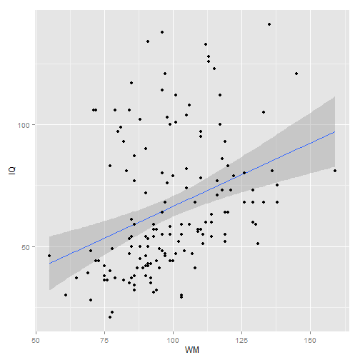
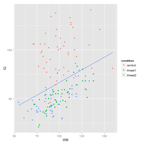
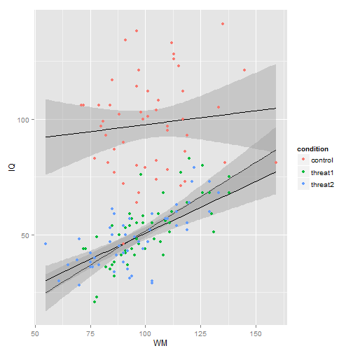
# Moderation analysis (uncentered): model_mod1 tests for 'first-order
# effects'; model_mod2 tests for moderation
model_mod1 <- lm(MOD$IQ ~ MOD$WM + MOD$D1 + MOD$D2)
summary(model_mod1)
Call:
lm(formula = MOD$IQ ~ MOD$WM + MOD$D1 + MOD$D2)

Residuals:
Min     1Q Median     3Q    Max
-47.34  -7.29   0.74   7.61  42.42


Coefficients:
Estimate Std. Error t value Pr(>|t|)
(Intercept)  59.7864     7.1436    8.37  4.3e-14 ***
MOD$WM        0.3728     0.0669    5.57  1.2e-07 ***
MOD$D1      -45.2055     2.9464  -15.34  < 2e-16 ***
MOD$D2      -46.9074     2.9922  -15.68  < 2e-16 ***
---
Signif. codes:  0 '***' 0.001 '**' 0.01 '*' 0.05 '.' 0.1 ' ' 1

Residual standard error: 14.7 on 146 degrees of freedom
Multiple R-squared:  0.725,	Adjusted R-squared:  0.719
F-statistic:  128 on 3 and 146 DF,  p-value: <2e-16
ggplot(MOD, aes(x = WM, y = IQ)) + geom_smooth(method = "lm") + geom_point()
ggplot(MOD, aes(x = WM, y = IQ)) + stat_smooth(method = "lm", se = F) + geom_point(aes(color = condition))
ggplot(MOD, aes(x = WM, y = IQ)) + geom_smooth(aes(group = condition), method = "lm",
se = T, color = "black", fullrange = T) + geom_point(aes(color = condition))
# Create new predictor variables
MOD$WM.D1 <- (MOD$WM * MOD$D1)
MOD$WM.D2 <- (MOD$WM * MOD$D2)
model_mod2 <- lm(MOD$IQ ~ MOD$WM + MOD$D1 + MOD$D2 + MOD$WM.D1 + MOD$WM.D2)
summary(model_mod2)
Call:
lm(formula = MOD$IQ ~ MOD$WM + MOD$D1 + MOD$D2 + MOD$WM.D1 +
MOD$WM.D2)

Residuals:
Min     1Q Median     3Q    Max
-50.41  -7.18   0.42   8.20  40.86


Coefficients:
Estimate Std. Error t value Pr(>|t|)
(Intercept)   85.585     11.358    7.54  5.0e-12 ***
MOD$WM         0.120      0.109    1.10   0.2730
MOD$D1       -93.095     16.857   -5.52  1.5e-07 ***
MOD$D2       -79.897     15.477   -5.16  8.0e-07 ***
MOD$WM.D1      0.472      0.164    2.88   0.0046 **
MOD$WM.D2      0.329      0.155    2.13   0.0353 *
---
Signif. codes:  0 '***' 0.001 '**' 0.01 '*' 0.05 '.' 0.1 ' ' 1

Residual standard error: 14.4 on 144 degrees of freedom
Multiple R-squared:  0.741,	Adjusted R-squared:  0.732
F-statistic: 82.4 on 5 and 144 DF,  p-value: <2e-16
anova(model_mod1, model_mod2)
Analysis of Variance Table

Model 1: MOD$IQ ~ MOD$WM + MOD$D1 + MOD$D2
Model 2: MOD$IQ ~ MOD$WM + MOD$D1 + MOD$D2 + MOD$WM.D1 + MOD$WM.D2
Res.Df   RSS Df Sum of Sq    F Pr(>F)
1    146 31655
2    144 29784  2      1871 4.52  0.012 *
---

Signif. codes:  0 '***' 0.001 '**' 0.01 '*' 0.05 '.' 0.1 ' ' 1
Mediation analysis
myCsv <- getURL("https://dl.dropboxusercontent.com/u/8272421/stat/stat_one_med.txt",
ssl.verifypeer = FALSE)
MED <- read.table(textConnection(myCsv), header = TRUE)
head(MED)
subject condition  IQ WM
1       1   control  73 37
2       2   control 128 77
3       3   control  83 32
4       4   control  83 33
5       5   control  64 53
6       6   control  95 46
# The function sobel in the multilevel package executes the entire mediation
# analysis in one step but first we will do it with 3 lm models
model.YX <- lm(MED$IQ ~ MED$condition)
model.YXM <- lm(MED$IQ ~ MED$condition + MED$WM)
model.MX <- lm(MED$WM ~ MED$condition)

summary(model.YX)
Call:
lm(formula = MED$IQ ~ MED$condition)

Residuals:
Min     1Q Median     3Q    Max
-35.32  -9.57  -1.82  10.68  39.68

Coefficients:
Estimate Std. Error t value Pr(>|t|)
(Intercept)            97.32       2.07   47.00  < 2e-16 ***
MED$conditionthreat   -11.00       2.93   -3.76  0.00029 ***
---

Signif. codes:  0 '***' 0.001 '**' 0.01 '*' 0.05 '.' 0.1 ' ' 1

Residual standard error: 14.6 on 98 degrees of freedom
Multiple R-squared:  0.126,	Adjusted R-squared:  0.117
F-statistic: 14.1 on 1 and 98 DF,  p-value: 0.000293
summary(model.YXM)
Call:
lm(formula = MED$IQ ~ MED$condition + MED$WM)

Residuals:
Min     1Q Median     3Q    Max
-31.88  -7.90   0.93   6.99  27.58

Coefficients:
Estimate Std. Error t value Pr(>|t|)
(Intercept)           55.998      4.644   12.06  < 2e-16 ***
MED$conditionthreat   -2.408      2.316   -1.04      0.3
MED$WM                 0.752      0.080    9.41  2.6e-15 ***
---

Signif. codes:  0 '***' 0.001 '**' 0.01 '*' 0.05 '.' 0.1 ' ' 1

Residual standard error: 10.6 on 97 degrees of freedom
Multiple R-squared:  0.543,	Adjusted R-squared:  0.533
F-statistic: 57.6 on 2 and 97 DF,  p-value: <2e-16
summary(model.MX)
Call:
lm(formula = MED$WM ~ MED$condition)

Residuals:
Min     1Q Median     3Q    Max
-31.92  -7.75  -0.50  10.18  30.50

Coefficients:
Estimate Std. Error t value Pr(>|t|)
(Intercept)            54.92       1.90   28.89  < 2e-16 ***
MED$conditionthreat   -11.42       2.69   -4.25  4.9e-05 ***
---

Signif. codes:  0 '***' 0.001 '**' 0.01 '*' 0.05 '.' 0.1 ' ' 1

Residual standard error: 13.4 on 98 degrees of freedom
Multiple R-squared:  0.156,	Adjusted R-squared:  0.147
F-statistic:   18 on 1 and 98 DF,  p-value: 4.91e-05
# Compare the results to the output of the sobel function
library(multilevel)
# Estimate Sobel's (1982) indirect test for mediation.  The function
# provides an estimate of the magnitude of the indirect effect, Sobel's
# first-order estimate of the standard error associated with the indirect
# effect, and the corresponding z-value.
model.ALL <- sobel(MED$condition, MED$WM, MED$IQ)
model.ALL
$`Mod1: Y~X`
Estimate Std. Error t value  Pr(>|t|)
(Intercept)    97.32      2.071  46.999 4.966e-69
predthreat    -11.00      2.928  -3.756 2.928e-04

$`Mod2: Y~X+M`
Estimate Std. Error t value  Pr(>|t|)
(Intercept)  55.9977      4.644  12.058 5.304e-21
predthreat   -2.4075      2.316  -1.039 3.012e-01
med           0.7524      0.080   9.406 2.577e-15

$`Mod3: M~X`
Estimate Std. Error t value  Pr(>|t|)
(Intercept)    54.92      1.901  28.895 9.487e-50
predthreat    -11.42      2.688  -4.249 4.906e-05

$Indirect.Effect
[1] -8.593

$SE
[1] 2.219

$z.value
[1] -3.872

$N
[1] 100
Conduct group comparisons with both parametric and non-parametric tests
myCsv <- getURL("https://dl.dropboxusercontent.com/u/8272421/stat/stat_one_t_anova.txt",
ssl.verifypeer = FALSE)
wm <- read.table(textConnection(myCsv), header = TRUE)
head(wm)
cond pre post gain train
1  t08   8    9    1     1
2  t08   8   10    2     1
3  t08   8    8    0     1
4  t08   8    7   -1     1
5  t08   9   11    2     1
6  t08   9   10    1     1
# Create two subsets of data: One for the control group and another for the
# training groups
wm.c = subset(wm, wm$train == "0")
wm.t = subset(wm, wm$train == "1")
# Dependent t-tests and Wilcoxan

# First, compare pre and post scores in the control group
t.test(wm.c$pre, wm.c$post, paired = T)
Paired t-test

data:  wm.c$pre and wm.c$post
t = -9.009, df = 39, p-value = 4.511e-11
alternative hypothesis: true difference in means is not equal to 0
95 percent confidence interval:
-2.418 -1.532
sample estimates:
mean of the differences
-1.975
# Wilcoxon Rank Sum and Signed Rank Tests Performs one- and two-sample
# Wilcoxon tests on vectors of data; the latter is also known as
# ‘Mann-Whitney’ test.
wilcox.test(wm.c$pre, wm.c$post, paired = T)
Wilcoxon signed rank test with continuity correction

data:  wm.c$pre and wm.c$post
V = 10, p-value = 1.717e-07
alternative hypothesis: true location shift is not equal to 0
# Next, compare pre and post scores in the training groups
t.test(wm.t$pre, wm.t$post, paired = T)
Paired t-test

data:  wm.t$pre and wm.t$post
t = -14.49, df = 79, p-value < 2.2e-16
alternative hypothesis: true difference in means is not equal to 0
95 percent confidence interval:
-3.966 -3.009
sample estimates:
mean of the differences
-3.487
# Wilcoxon
wilcox.test(wm.t$pre, wm.t$post, paired = T)
Wilcoxon signed rank test with continuity correction

data:  wm.t$pre and wm.t$post
V = 10, p-value = 3.017e-14
alternative hypothesis: true location shift is not equal to 0
# Cohen's d for dependent t-tests
library(lsr)
cohensD(wm.c$post, wm.c$pre, method = "paired")
[1] 1.424
cohensD(wm.t$post, wm.t$pre, method = "paired")
[1] 1.62
# Independent t-test and Mann Whitney

# Compare the gain scores in the control and training groups
t.test(wm$gain ~ wm$train, var.equal = T)
Two Sample t-test

data:  wm$gain by wm$train
t = -4.04, df = 118, p-value = 9.539e-05
alternative hypothesis: true difference in means is not equal to 0
95 percent confidence interval:
-2.2538 -0.7712
sample estimates:
mean in group 0 mean in group 1
1.975           3.487
# Mann-Whitney
wilcox.test(wm$gain ~ wm$train, paired = F)
Wilcoxon rank sum test with continuity correction

data:  wm$gain by wm$train
W = 916, p-value = 0.0001061
alternative hypothesis: true location shift is not equal to 0
# Cohen's d for independent t-tests
cohensD(wm$gain ~ wm$train, method = "pooled")
[1] 0.7824
# Analysis of Variance (ANOVA) and Kruskul Wallis To compare the gain scores
# across all groups, use ANOVA First, check the homogeneity of variance
# assumption
library(car)
leveneTest(wm.t$gain, wm.t$cond, center = "mean")
Levene's Test for Homogeneity of Variance (center = "mean")
Df F value Pr(>F)
group  3    1.13   0.34
76
leveneTest(wm.t$gain, wm.t$cond)
Levene's Test for Homogeneity of Variance (center = median)
Df F value Pr(>F)
group  3    1.31   0.28
76
aov.model = aov(wm.t$gain ~ wm.t$cond)
summary(aov.model)
Df Sum Sq Mean Sq F value  Pr(>F)
wm.t$cond    3    213      71    35.3 2.2e-14 ***
Residuals   76    153       2
---

Signif. codes:  0 '***' 0.001 '**' 0.01 '*' 0.05 '.' 0.1 ' ' 1
# Kruskal Wallis Rank Sum Test
kruskal.test(wm.t$gain ~ wm.t$cond)
Kruskal-Wallis rank sum test

data:  wm.t$gain by wm.t$cond
Kruskal-Wallis chi-squared = 50.25, df = 3, p-value = 7.084e-11
# Effect size for ANOVA
etaSquared(aov.model, anova = T)
eta.sq eta.sq.part    SS df     MS     F         p
wm.t$cond 0.5821      0.5821 213.0  3 71.013 35.29 2.154e-14
Residuals 0.4179          NA 152.9 76  2.012    NA        NA
# Conduct post-hoc tests to evaluate all pairwise comparisons
TukeyHSD(aov.model)
Tukey multiple comparisons of means
95% family-wise confidence level

Fit: aov(formula = wm.t$gain ~ wm.t$cond)

$`wm.t$cond`
diff    lwr   upr  p adj
t12-t08 1.25 0.0716 2.428 0.0333
t17-t08 3.05 1.8716 4.228 0.0000
t19-t08 4.25 3.0716 5.428 0.0000
t17-t12 1.80 0.6216 2.978 0.0008
t19-t12 3.00 1.8216 4.178 0.0000
t19-t17 1.20 0.0216 2.378 0.0443
Conduct a binary logisitc regression
myCsv <- getURL("https://dl.dropboxusercontent.com/u/8272421/stat/stat_one_glm.txt",
ssl.verifypeer = FALSE)
BL <- read.table(textConnection(myCsv), header = TRUE)
head(BL)
subject verdict danger rehab punish gendet specdet incap
1       1       0      2     2      2      2       0     7
2       2       0      0     9      0      6       8     2
3       3       1      6     3      2     10      10     4
4       4       1      1     3      2      3       2     1
5       5       0      0     7      4      1       1    10
6       6       1     10     6      1      8       0     0
# Binary logistic regression
lrfit <- glm(BL$verdict ~ BL$danger + BL$rehab + BL$punish + BL$gendet + BL$specdet +
BL$incap, family = binomial)
summary(lrfit)
Call:
glm(formula = BL$verdict ~ BL$danger + BL$rehab + BL$punish +
BL$gendet + BL$specdet + BL$incap, family = binomial)

Deviance Residuals:
Min      1Q  Median      3Q     Max
-1.969  -0.932  -0.463   0.891   1.957

Coefficients:
Estimate Std. Error z value Pr(>|z|)
(Intercept) -1.74758    0.91728   -1.91   0.0568 .
BL$danger    0.29339    0.09292    3.16   0.0016 **
BL$rehab    -0.18784    0.08140   -2.31   0.0210 *
BL$punish    0.07012    0.07111    0.99   0.3241
BL$gendet    0.18574    0.07733    2.40   0.0163 *
BL$specdet   0.00590    0.07865    0.08   0.9402
BL$incap     0.00353    0.07587    0.05   0.9629
---

Signif. codes:  0 '***' 0.001 '**' 0.01 '*' 0.05 '.' 0.1 ' ' 1

(Dispersion parameter for binomial family taken to be 1)

Null deviance: 138.47  on 99  degrees of freedom
Residual deviance: 114.06  on 93  degrees of freedom
AIC: 128.1

Number of Fisher Scoring iterations: 3
confint(lrfit) # CIs using profiled log-likelihood (default for logistic models)
2.5 %   97.5 %
(Intercept) -3.65201 -0.02217
BL$danger    0.11998  0.48756
BL$rehab    -0.35426 -0.03283
BL$punish   -0.06763  0.21352
BL$gendet    0.03858  0.34394
BL$specdet  -0.15006  0.16092
BL$incap    -0.14735  0.15284
confint.default(lrfit) # CIs using standard errors
2.5 %   97.5 %
(Intercept) -3.54542  0.05027
BL$danger    0.11127  0.47550
BL$rehab    -0.34738 -0.02831
BL$punish   -0.06926  0.20950
BL$gendet    0.03418  0.33730
BL$specdet  -0.14824  0.16005
BL$incap    -0.14518  0.15224
# Model fit
with(lrfit, null.deviance - deviance)  #difference in deviance for the two models
[1] 24.41
with(lrfit, df.null - df.residual) #df for the difference between the two models
[1] 6
with(lrfit, pchisq(null.deviance - deviance, df.null - df.residual, lower.tail = FALSE)) #p-value
[1] 0.0004397
# Wald tests for Model Coefficients Computes a Wald chi-squared test for 1
# or more coefficients, given their variance-covariance matrix.
library(aod)
wald.test(b = coef(lrfit), Sigma = vcov(lrfit), Terms = 2)  #danger
Wald test:
----------

Chi-squared test:
X2 = 10.0, df = 1, P(> X2) = 0.0016
wald.test(b = coef(lrfit), Sigma = vcov(lrfit), Terms = 3) #rehab
Wald test:
----------


Chi-squared test:
X2 = 5.3, df = 1, P(> X2) = 0.021
wald.test(b = coef(lrfit), Sigma = vcov(lrfit), Terms = 4) #punish
Wald test:
----------

Chi-squared test:
X2 = 0.97, df = 1, P(> X2) = 0.32
wald.test(b = coef(lrfit), Sigma = vcov(lrfit), Terms = 5) #gendet
Wald test:
----------


Chi-squared test:
X2 = 5.8, df = 1, P(> X2) = 0.016
wald.test(b = coef(lrfit), Sigma = vcov(lrfit), Terms = 6) #specdet
Wald test:
----------

Chi-squared test:
X2 = 0.0056, df = 1, P(> X2) = 0.94
wald.test(b = coef(lrfit), Sigma = vcov(lrfit), Terms = 7) #incap
Wald test:
----------


Chi-squared test:
X2 = 0.0022, df = 1, P(> X2) = 0.96
# Odds ratios
exp(coef(lrfit))  #exponentiated coefficients
(Intercept)   BL$danger    BL$rehab   BL$punish   BL$gendet  BL$specdet
0.1742      1.3410      0.8287      1.0726      1.2041      1.0059
BL$incap
1.0035
# Classification table
library(QuantPsyc)
# Provides a Classification analysis for a logistic regression model.  Also
# provides McFadden's Rsq.
ClassLog(lrfit, BL$verdict)
$rawtab
resp
0  1
FALSE 39 16
TRUE  13 32

$classtab
resp
0      1
FALSE 0.7500 0.3333
TRUE  0.2500 0.6667

$overall
[1] 0.71

$mcFadden
[1] 0.1763
Statistics One is available on coursera