library(plyr)
library(ggplot2)
Example data
library(RCurl)
myCsv <- getURL("https://dl.dropboxusercontent.com/u/8272421/bnames.csv", ssl.verifypeer = FALSE)
myData <- read.csv(textConnection(myCsv))

myData$name = as.character(myData$name)
myData$sex = as.character(myData$sex)
head(myData)
year    name percent sex
1 1880    John 0.08154 boy
2 1880 William 0.08051 boy
3 1880   James 0.05006 boy
4 1880 Charles 0.04517 boy
5 1880  George 0.04329 boy
6 1880   Frank 0.02738 boy
transform() modifies an existing data frame.
Define functions
# get the nth character
letter <- function(x, n = 1) {
if (n < 0) {
nc <- nchar(x)
n <- nc + n + 1
}
tolower(substr(x, n, n))
}

# get the number of vowels
vowels <- function(x) {
nchar(gsub("[^aeiou]", "", x))
}
Simple transformation
bnames = myData
bnames0 <- transform(bnames, first = letter(name, 1), last = letter(name, -1),
length = nchar(name), vowels = vowels(name))
head(bnames0)
year    name percent sex first last length vowels
1 1880    John 0.08154 boy     j    n      4      1
2 1880 William 0.08051 boy     w    m      7      3
3 1880   James 0.05006 boy     j    s      5      2
4 1880 Charles 0.04517 boy     c    s      7      2
5 1880  George 0.04329 boy     g    e      6      3
6 1880   Frank 0.02738 boy     f    k      5      1
Group-wise transformation
compute the rank of a name within a sex and year (e.g. boy & 2008)?
one <- subset(myData, sex == "boy" & year == 2008)
# ties.method = 'first' -- first occurrence wins
one <- transform(one, rank = rank(-percent, ties.method = "first"))
head(one)
year      name  percent sex rank
128001 2008     Jacob 0.010355 boy    1
128002 2008   Michael 0.009437 boy    2
128003 2008     Ethan 0.009301 boy    3
128004 2008    Joshua 0.008799 boy    4
128005 2008    Daniel 0.008702 boy    5
128006 2008 Alexander 0.008566 boy    6
Transform every sex and year
# short the data to easily see the results
bnames = myData[c(1:2, 9999:10000, 129001:129002, 257998:258000), ]
bnames
year    name  percent  sex
1      1880    John 0.081541  boy
2      1880 William 0.080511  boy
9999   1889  Collie 0.000042  boy
10000  1889  Cooper 0.000042  boy
129001 1880    Mary 0.072381 girl
129002 1880    Anna 0.026678 girl
257998 2008  Kenley 0.000127 girl
257999 2008  Sloane 0.000127 girl
258000 2008 Elianna 0.000127 girl
# rank by sex and then by year
bnames1 <- ddply(bnames, c("sex", "year"), transform, rank = rank(-percent,
ties.method = "first"))
bnames1
year    name  percent  sex rank
1 1880    John 0.081541  boy    1
2 1880 William 0.080511  boy    2
3 1889  Collie 0.000042  boy    1
4 1889  Cooper 0.000042  boy    2
5 1880    Mary 0.072381 girl    1
6 1880    Anna 0.026678 girl    2
7 2008  Kenley 0.000127 girl    1
8 2008  Sloane 0.000127 girl    2
9 2008 Elianna 0.000127 girl    3
# rank by yaer and then by sex
bnames2 <- ddply(bnames, c("year", "sex"), transform, rank = rank(-percent,
ties.method = "first"))
bnames2
year    name  percent  sex rank
1 1880    John 0.081541  boy    1
2 1880 William 0.080511  boy    2
3 1880    Mary 0.072381 girl    1
4 1880    Anna 0.026678 girl    2
5 1889  Collie 0.000042  boy    1
6 1889  Cooper 0.000042  boy    2
7 2008  Kenley 0.000127 girl    1
8 2008  Sloane 0.000127 girl    2
9 2008 Elianna 0.000127 girl    3
summarise() creates a new data frame.
Simple summaries
Whole dataset summaries
summarise(bnames, max_perc = max(percent), min_perc = min(percent))
max_perc min_perc
1  0.08154  4.2e-05
Group-wise summaries
bnames = bnames0

sum.name = ddply(bnames, c("name"), summarise, tot = sum(percent))
head(sum.name)
name      tot
1   Aaden 0.000442
2 Aaliyah 0.019748
3   Aarav 0.000101
4   Aaron 0.293097
5      Ab 0.000218
6 Abagail 0.001326
sum.length = ddply(bnames, c("length"), summarise, tot = sum(percent))
head(sum.length)
length     tot
1      2  0.2315
2      3  7.2744
3      4 36.8475
4      5 57.7588
5      6 60.3609
6      7 44.3370
sum.year.sex = ddply(bnames, c("year", "sex"), summarise, tot = sum(percent))
head(sum.year.sex)
year  sex    tot
1 1880  boy 0.9307
2 1880 girl 0.9345
3 1881  boy 0.9304
4 1881 girl 0.9327
5 1882  boy 0.9275
6 1882 girl 0.9310
sum.sex.year = ddply(bnames, c("sex", "year"), summarise, tot = sum(percent))
head(sum.sex.year)
sex year    tot
1 boy 1880 0.9307
2 boy 1881 0.9304
3 boy 1882 0.9275
4 boy 1883 0.9288
5 boy 1884 0.9273
6 boy 1885 0.9255
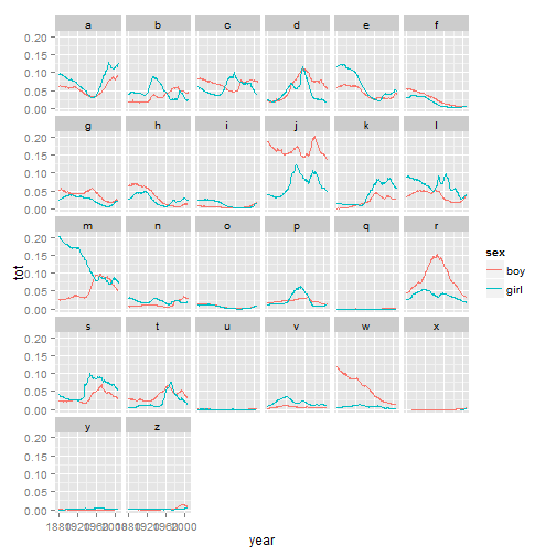
The proportion of the first letter (by year)
sum.year.sex.first <- ddply(bnames, c("year", "sex", "first"), summarise, tot = sum(percent))
qplot(year, tot, data = sum.year.sex.first, geom = "line", colour = sex, facets = ~first)
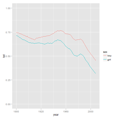
The proportion of US children who have a name in the top 100 (by year)
# rank by sex and then by year
bnames = myData
bnames = ddply(bnames, c("sex", "year"), transform, rank = rank(-percent, ties.method = "first"))
# top 100
top100 <- subset(bnames, rank <= 100)
top100s <- ddply(top100, c("sex", "year"), summarise, tot = sum(percent))
qplot(year, tot, data = top100s, colour = sex, geom = "line", ylim = c(0, 1))
ddply
Simple example
top100 <- subset(bnames, rank <= 100)
top100s <- ddply(top100, c("sex", "year"), summarise, tot = sum(percent))
head(top100s)
sex year    tot
1 boy 1880 0.7478
2 boy 1881 0.7466
3 boy 1882 0.7416
4 boy 1883 0.7438
5 boy 1884 0.7387
6 boy 1885 0.7342
ddply with your own defined function
One simple function
top100m <- ddply(top100, c("sex", "year"), function(df) mean(df$percent))
head(top100m)
sex year       V1
1 boy 1880 0.007478
2 boy 1881 0.007466
3 boy 1882 0.007416
4 boy 1883 0.007438
5 boy 1884 0.007387
6 boy 1885 0.007342
More than one function
top100ms <- ddply(top100, c("sex", "year"), function(df) c(mean(df$percent),
sd(df$percent)))
head(top100ms)
sex year       V1      V2
1 boy 1880 0.007478 0.01381
2 boy 1881 0.007466 0.01361
3 boy 1882 0.007416 0.01320
4 boy 1883 0.007438 0.01313
5 boy 1884 0.007387 0.01268
6 boy 1885 0.007342 0.01241
Set the column names
top100ms2 <- ddply(top100, c("sex", "year"), function(df) data.frame(mean = mean(df$percent),
se = sd(df$percent)/sqrt(length(df$percent))))
head(top100ms2)
sex year     mean       se
1 boy 1880 0.007478 0.001381
2 boy 1881 0.007466 0.001361
3 boy 1882 0.007416 0.001320
4 boy 1883 0.007438 0.001313
5 boy 1884 0.007387 0.001268
6 boy 1885 0.007342 0.001241
xxply
array dataFrame  list
array     aaply     adply alply
dataFrame daply     ddply dlply
list      laply     ldply llply