NCCTG Lung Cancer Data
Description: Survival in patients with advanced lung cancer from the North Central Cancer Treatment Group. Performance scores rate how well the patient can perform usual daily activities.
library(survival)
data(lung)
head(lung)
  inst time status age sex ph.ecog ph.karno pat.karno meal.cal wt.loss
1    3  306      2  74   1       1       90       100     1175      NA
2    3  455      2  68   1       0       90        90     1225      15
3    3 1010      1  56   1       0       90        90       NA      15
4    5  210      2  57   1       1       90        60     1150      11
5    1  883      2  60   1       0      100        90       NA       0
6   12 1022      1  74   1       1       50        80      513       0
inst:       Institution code
time:       Survival time in days
status:     censoring status 1=censored, 2=dead
age:        Age in years
sex:        Male=1 Female=2
ph.ecog:    ECOG performance score (0=good 5=dead)
ph.karno:   Karnofsky performance score (bad=0-good=100) rated by physician
pat.karno:  Karnofsky performance score as rated by patient
meal.cal:   Calories consumed at meals
wt.loss:    Weight loss in last six months
# Kaplan-Meier Analysis
Estimate survival-function
Global Estimate
km.as.one <- survfit(Surv(time, status) ~ 1,
                     type="kaplan-meier",
                     conf.type="log",
                     data=lung)
separate estimate for all sex
km.by.sex <- survfit(Surv(time, status) ~ sex,
                     type="kaplan-meier",
                     conf.type="log", data=lung)
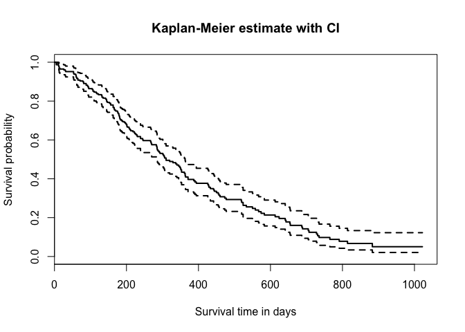
Plot estimated survival function
plot(km.as.one, main="Kaplan-Meier estimate with CI",
     xlab="Survival time in days",
     ylab="Survival probability", lwd=2)
plot(km.by.sex, main="Kaplan-Meier estimate by sex",
     xlab="Survival time in days",
     ylab="Survival probability",
     lwd=2, col = c("red","blue"))
legend(x="topright", col=c("red","blue"), lwd=2,
       legend=c("male","female"))

Plot cumulative incidence function
plot(km.by.sex, main="Kaplan-Meier cumulative incidence by sex",
     xlab="Survival time in days", ylab="Cumulative incidence",
     lwd=2, col = c("red","blue"),
     fun = function(x){1-x})
legend(x="bottomright", col=c("red","blue"),
       lwd=2, legend=c("male","female"))

Plot cumulative hazard
plot(km.as.one, main="Kaplan-Meier estimate",
     xlab="Survival time in days",
     ylab="Cumulative hazard", lwd=2,
     fun="cumhaz")

Log-rank-test for equal survival-functions
With rho = 0 (default) this is the log-rank or Mantel-Haenszel test, and with rho = 1 it is equivalent to the Peto & Peto modification of the Gehan-Wilcoxon test.
survdiff(Surv(time, status) ~ sex, data=lung)
Call:
survdiff(formula = Surv(time, status) ~ sex, data = lung)

        N Observed Expected (O-E)^2/E (O-E)^2/V
sex=1 138      112     91.6      4.55      10.3
sex=2  90       53     73.4      5.68      10.3

 Chisq= 10.3  on 1 degrees of freedom, p= 0.00131